Probability and Statistics (Part1. Intro to Probability)

Posted on 2023-12-30 Edited on 2024-09-19 In Notes Views: Word count in article: 10k Reading time ≈ 9 mins.

Probability and statistics is an essential tool to analyze and study data and construct mathematical models to make decisions and evaluations. This note will encompass a wide range of probability and statictical problems related to real-life applications by refering to several classical probability textbooks and materials, for example, A First Course to Probability by Sheldon M. Ross, An Introduction to Mathematical Statistics and Its Applications by Richard J. Larsen, Probability and Mathematical Statistics by Chen Xiru, and Harvad 110: Intro to Probability

And it's time to roll the dice.

Elementary Probability

Basic Principles of Counting

Permutation and Combination

Def: Given $n$ objects,

Permutation of $k$ objects: $A^n_k=\dfrac{n!}{(n-k)!}$

Combination of $k$ objects: $\tbinom{n}{k}=\dfrac{n!}{(n-k)!k!}=\dfrac{k(k-1)(k-2)...(k-n+1)}{n!}$

Story proof of combination identies

$\tbinom{n}{k}k=n\tbinom{n-1}{k-1}$. Pick $k$ people out of $n$ with 1 desginated as the President.

The left hand side means"first pick $k$ people out of $n$ then choose the President, while the right hand side says "first pick a President then pick $k-1$ people from $n-1$ remaining people, grouped with he selected President. They are equivalent.

Vandermende's Identity: $\tbinom{m+n}{k}=\sum_{j=0}^k\tbinom{m}{j}\tbinom{n}{k-j}$. Pick total $k$ items from 2 groups, one with $m$ items and the other with $n$.
$\tbinom{n}{r} = \tbinom{n-1}{r-1} + \tbinom{n-1}{r}$
Induction proof of binomial theorem:

n entries m 1s

m = 2

1 _ _ _ _ _ n-2

_ 1 _ _ _ _ n-3

_ _ 1 _ _ _ n-3

_ _ 1 _ _

(n-2) (n-3) + (n-2)*2 = (n-2)(n-1)

Birthday Problem (naive probability theory)

How big the group should be if the probability of at least two people in the group have the same birthday? Assume the group has $k$ people in total.

if $k>365$, $P = 1$.
if k< 365, consider 365 boxes representing the dates, then the people select the box (birthday) one by one.

$P(\mathrm{no-match})=\dfrac{365}{365}\dfrac{364}{365}\dfrac{363}{365}...\dfrac{365-k+1}{365}$

$P(\mathrm{match})=1-\dfrac{365...(365-k+1)}{365^k}$

Simulation:

R
Python

replicate the experiment for 10^4 times, for each time, we tabulate the sample result of $P^{365}_{23}.$ If the maximum number in the tabulated table is bigger than 2, then it is counted as success.

1 2	r <- replicate(10^4, max(tabulate(sample(1:365,23,replace=TRUE)))) sum(r>=2)/10^4

import random
import matplotlib.pyplot as plt

def birthday(k):
    birthday=[0]*365
    for i in range(k):
        birthday[random.randint(0,364)]+=1
    for i in range(365):
        if (birthday[i] >= 2):
            return 1
    return 0
        
def simulation(times,k):
    success=0
    for i in range(times):
        success += birthday(k)
    return success/times

def plot_sim(times,k_max):
    k_list = range(k_max)
    sim_list = [0]*k_max
    for i in range(k_max):
        sim_list[i] = simulation(times,k_list[i])
    plt.plot(k_list,sim_list)

if __name__ == "__main__":  
    plot_sim(1000,200)
    plt.show()

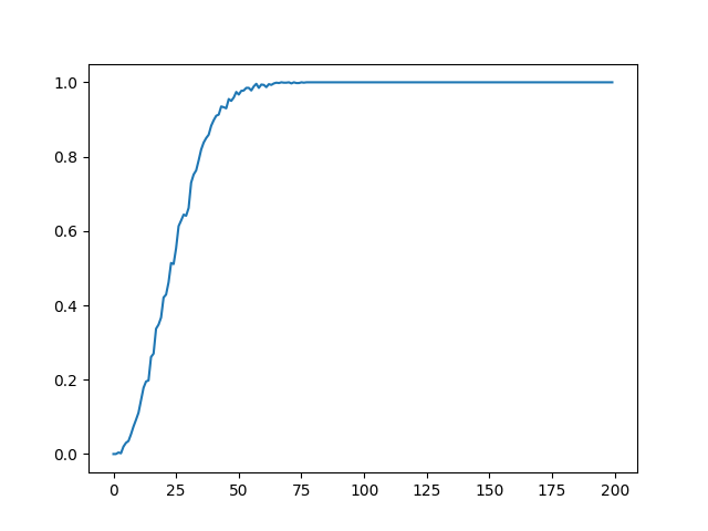The probability is almost one after k goes over 50.

Probability Measures and Spaces

Def: Let $S$ be a sample space and $F$ a sigma-field on $S$. Then a function \[ P:F\rightarrow[0,1],\space\space\space A\rightarrow P[A],\nonumber \] is called a probability measure on $S$ if

$P[S]=1$.

and (2) For any set of events ${A_k}$ such that $A_jA_k = $ for $j\neq k$, \[ P[\bigcup_kA_k]=\sum_kP[A_k]\nonumber \] Then $S$ is called a probability space

This is a formal definition of a probability measures and spaces in an axiomatic approach. Here sigma field is defined as a collection of sets that hold following properties:

If the subset $A$ is in the sigma-field, then so is its complement $A^c$.
If $A_n$ are countably infinitely many subsets from the sigma-field, then both the intersection and union of all of these sets is also in the sigma-field.

Inclusion and Exclusion

\[P(A_1 \cup A_2 ... \cup A_n)=\sum_{j=1}^nP(A_j)-\sum_{i<j}P(A_i\cap A_j)+\sum_{1<j<k}P(A_1\cap A_j\cap A_k)+(-1)^{n+1}P(A_1\cap...\cap A_n).\]

The practical way of using the terrible equation above is to calculate each term seperately and pay attention to the pattern of the middle joint terms. It is oftern used in "matching problems", and it divides a big problem into smaller ones.

de Montmort's Problem (1713)

Consider a well shuffled deck of n cards labelled 1 through n. You flip over the cards one by one, saying the numbers 1 through n as you do so. You win the game if, at some point, the number you say aloud is the same as the number on the number on the card being flipped over (for example, if the 8th card in the deck has the label 8). What is the probability of winning?

Let $A_j$ be the event that "jth card matches". Then we are interested in \[ P(\bigcup_{j=1}^n A_j)=? \] Consider separete events. The simpler problem can be interpreted as "the probability of the card with number j sitts on the jth position".

\[P(A_j)=\dfrac{1}{n}, \quad P(A_1\cap A_2)=\dfrac{1}{ n (n-1) },\quad P(A_1\cap A_2 ...\cap A_k)=\dfrac{1}{ n (n-k+1) }\nonumber\]

Then consider the coefficients: the summation symbol can be written as: $\tbinom{n}{k}$, then we have:

\[P(\bigcup_{j=1}^n A_j)=n\cdot\dfrac{1}{n}-\dfrac{n(n-1)}{2! }\dfrac{1}{ n(n-1) }+\dfrac{ n(n-1)(n-2) }{3!}\dfrac{1}{ n(n-1)(n-2) }+...=1-\dfrac{1}{2! }+\dfrac{1}{3!}-...+(-1)^n\dfrac{1}{n! }=1-\dfrac{1}{e}\]

The last equation holds as $n$ is large enough from Taylor Series.

Conditional Probability

Conditioning is the soul of statistics

Conditional probability can be of great importance, as it can help us calculate probabilities when some partial information is provided, and it also derives the Baye's Theroem.

Def: if\[P(B)>0\], then \[ P(A|B)=\dfrac{P(A\cap B)}{P(B) }. \] The denominator \[P(B)\] suggests that the conditional probability actually narrow the sample space into a subspace of the original space, therefore increasing the probability in question. In other words, the given conditions can help us eliminate some events that do not meet the condition, adding to the possibility of the event we want.

Here comes the exam

A student is taking a one-hour-time-limit makeup examination. Suppose the probability that the student will finish the exam in less than $x$ hours is $x/2 $, for all $0\leq x\leq 1$. Then, given that the student is still working after 0.75 hour, what is the conditional probability that the full hour is used?

sol: let $A$ be the event that the student use the full hour, i.e. not finish the exam in one hour. And $B$ be the condition that the student is still working after 0.75 hour. \[ P(A|B)=\dfrac{P(A\cap B) }{P(B)}=\dfrac{1-1/2}{1-0.75/2}=0.8 \] Notice:

$P(A\cap B)=P(A)$ is because $A$ and $B$ are actually the complement of the given $x/2$ relation, therefore $A\subseteq B.$

Law of Total Probability

Let $A_n$ be a total partition, $B$ be an event of space $A$, then \[ P(B)=P(B\cap A_1)+P(B\cap A_2)+...P(B\cap A_n)=\sum_{i=1}^nP(B|A_i)P(A_i) \] One of the most famous problems regarding LOTP is the Monty Hall Problem.

Monty Hall

Given three doors, among which one door has a car, two doors hide goats. A goat door is always opened by Monty with equal probability. Should you switch the door after you select and Monty opens one?

Intuition:

One way to think this problem in intuition is to consider there are 10000 doors, and therefore our intuition is that the chance of selecting the correct door(the door has car) at the first place is very small. After the monty opens 9998 doors, namely helping us eliminate 9998 wrong answers, we are sufficient to switch.

Law of Total Probability

Let $S$ denotes the event that we switch to the right door. $D_j$ be the event that the car is in door $j$. Suppose we first choose door $1$.

Then $P(S)=(P(S|D_1)+P(S|D_2)+P(S|D_3))\dfrac{1}{3}=(0+1+1)\dfrac{1}{3}=\dfrac{2}{3}$. For $P(S|D_j)$, consider we switch from door $1$ to door $j$.

Tree graph

In such finite problem with different scenarios, we can also use tree graph to show the whole process.

Simulation

import random
from random import choice
import matplotlib as plt

def monty_hall(n_door):
# setup
    car_index = random.randint(0,n_door-1)
    choose_index = random.randint(0,n_door-1)

    def choose(n_door, chosen_index, choose_index, list):
        for i in range(0,n_door):
            if i != chosen_index and i != choose_index:
                list.append(i)
        return choice(list)

    open_index_list = []
    monty_index = choose(n_door, car_index, choose_index, open_index_list)
    switch_index_list = []
    switch_index = choose(n_door, monty_index, choose_index, switch_index_list)

    return 1 if switch_index == car_index else 0

def simulation(time):
    success = 0
    for i in range(time):
        success += monty_hall(3)
    return success/time

if __name__ == "__main__":
    print(simulation(10000))
    
0.6722

\[\begin{align} \end{align}\]