Linear Algebra (Part I. Linear Equations)
It's a little bit strange to put linear algebra and functions of multiple variables together. However, they are highly related in their essence. Functions of multiple variables take advantage of derivative to change a complicated function into a linear one, which can be further analyzed with linear algebra.
And so the adventure begins...
Solving Linear Equations
Linear Equations
A linear equation with \(n\) unknowns is an eaquation like this: \[ a_1x_1+a_2x_2+\cdots+a_nx_n=b \] The unknowns should be multiplied by only numbers and never will we see \(xy\) or \(x^2\). Therefore, we can see that: \(4x_1-5x_2=x_1x_2\) and \(x_2=2\sqrt{x_1}-6\) are not linear equations as the former has \(x_1x_2\), while the latter has \(\sqrt{x_1}\).
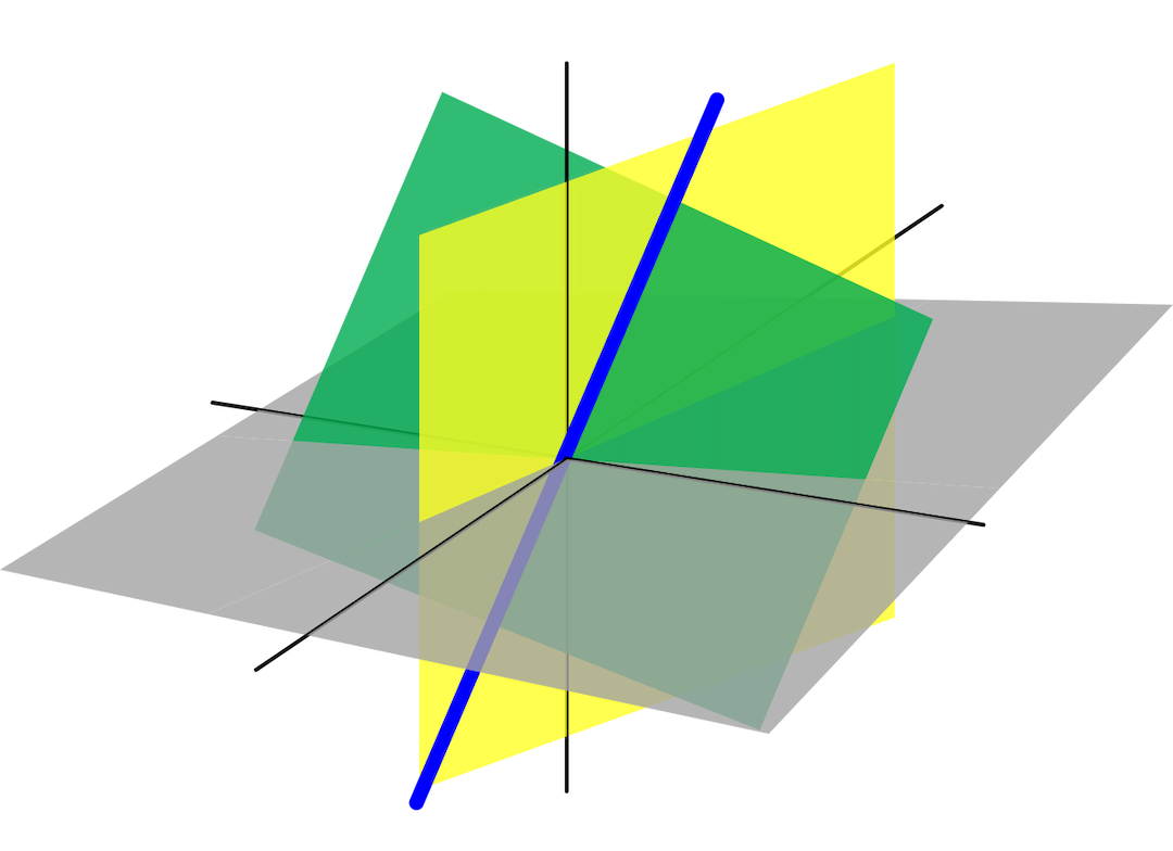
We can get a linear equation system by combining several linear equations together. Let's start from this example: \[ \begin{aligned} x-2y&=1 \\\ 3x+2y&=11 \end{aligned} \]
Row Picture
The row picture of linear equations can be seen as lines in a coordinate;
Column Picture
The column picture sees vectors instead of numbers. \[ \begin{pmatrix}1\\3\end{pmatrix}x+\begin{pmatrix}-2\\2\end{pmatrix}y=\begin{pmatrix}1\\11\end{pmatrix} \] We can get a linear combination if we take \(x=3,y=1\). \[ 3 \begin{pmatrix} 1\\ 3\end{pmatrix}+ \begin{pmatrix} -2\\ 2\end{pmatrix} = \begin{pmatrix} 1 \\11\end{pmatrix} \]
Consistent and Inconsistent
A system of linear equations has
- no solution
- only one solution
- infinitely many solutions
Consistent:one solution or infinite solutions
Inconsistent: No solution
Matrix
The main information in a linear system can be represented by a matrix, a chart of numbers.
If we put the coefficients together, then we have a coefficient matrix: \[ \left [ \begin{array}{rrrr} 1&-2\\ 3&2\\ \end{array} \right ] \] If we include the numbers on the right hand side of the equations, we will have an augumented matrix: \[ \left [ \begin{array}{rrrr} 1&-2&1\\ 3&2&11\\ \end{array} \right ] \] The rigiorous definition of a matrix can be written as follows:
Definition of Matrices
Let \(m\) and \(n\) denote positive integers. An \(m\)-by-\(n\) matrix A is a rectangular array of elements of \(\mathbf{F}\) with \(m\) rows and \(n\) columns: \[ A=\begin{bmatrix} a_{11}&...&a_{1n}\\ \vdots&\ddots&\vdots\\ a_{m1}&...&a_{mn} \end{bmatrix} \] And the notation \(A_{jk}\) denotes the entry in row \(j\),column \(k\) of \(A\).
The real meaning of matrices is more abstract and comlicated than just a simple "rectangular array of elements". Anyway, we will talk it later.
The idea of elimination
To slove linear equations, the main idea is elimination. Before elimination, \(x\) and \(y\) Appear in both equations. After elimintaion, \(y\) has disappeared leaving \(x\) alone.
There are three ways to deal with linear equations:
Elementary Row Transformation
- (Replacement) substitue an equation with the sum of itself and another equation multiplied with a scalar.
- (Interchange) change the position of two equations.
- (Scaling) multiply an equation with a non-zero scalar.
One principle we can use: determine the pivot and make the entry below zero.
Matrix Multiplication
The first thing to do before you multiply two matrices is to check whether they can multiply. \[ A_{m\times n}B_{n\times p}=C_{m\times p} \] Then the output of matrix multiplication can be expressed as follows:
Each entry in \(AB=C\) is a dot product: \(C_{ij}=\) (row \(i\) of \(A\))\(\cdot\)(column \(j\) of \(B\))
or you can write it in a more mathematical way: \[ C_{ij}=\sum\limits_{k=1}^nA_{ik}B_{kj} \]
Properties of Matrix Multiplication
- \(A(BC)=(AB)C\)
- \(A(B+C)=AB+AC\)
- \((B+C)A=BA+CA\)
- \(\forall r,\space r(AB)=(rA)B=A(rB)\)
The real meaning of matrix multiplication will be discussed after we introduce linear transformation.
The Matrix Equation \(Ax=b\)
A fundamental idea in linear algebra is to view a linear combination of vectors as the product of a matrix and a vector. Therefore, we can immediately write linear equations into a matrix equation:
Suppose that \(x=[x_1,x_2,\cdots,x_n]^T\) and \(A= [a_{11},a_{12},\cdots,a_{1n}]^T\), then the linear equation can be written as: \[ Ax=b \]
Now we have turned a linear equation into a matrix equation. The target has become a simple \(x\). To take advantage of this equation, we need inverse matrices.
Inverse Matrices
Suppose \(A\) is a square matrix (so we can deal with it more easily). The inverse matrix of \(A\) is denoted as \(A^{-1}\), which undoes whatever \(A\) does. There product should be identity matrix \(I\), doing nothing to the original matrix. We have the following relation
Inverse Matrices
The matrix \(A\) is invertible if there exists a matrix \(A^{-1}\) that "inverts" \(A\). \[ A^{-1}A=I=AA^{-1} \]
There are also some properties of inverse matrices and matrix multiplications:
Reverse of product
\[ (AB)^{-1}=B^{-1}A^{-1} \]
Proof: \[ (AB)(B^{-1}A^{-1})=AIA^{-1}=I \] To prove a "reverse equation", a practical method is to take the both side of the equation together.
The solution of \(Ax=b\)
With the help of inverse matrices, we can immediately get \(x\) \[ A^{-1}Ax=A^{-1}b\\ x=A^{-1}b \] As \(b\) is something we know, so the whole problem has changed from "find \(x\)" to "find \(A^{-1}\)". However, not all matrices have inverses. Here are some notes about \(A^{-1}\).
Notes for the solution \(A^{-1}\):
The inverse exists if and only if elimination prodces \(n\) pivots.
The matrix \(A\) Cannot have two "solutions".
Suppose there exists another inverse \(B\), then \[ B(AA^{-1})=(BA)A^{-1}\Rightarrow BI=IA^{-1}\Rightarrow B=A^{-1} \]
Suppose there is a nonzero vector \(x\) such that \(Ax=0\), Then \(A\) cannot have an inverse. If \(A\) is invertible, then \(Ax=0\) can only have the zero solution \(x=A^{-1}0=0\).
A 2 by 2 matrix is invertible if and only if \(ad-bc\), the \(\det A\) is not zero. And the inverse interchanges the leading diagonal and add "\(-\)" to the minus diagonal.
\[ \begin{bmatrix} a&b\\ c&d\\ \end{bmatrix} ^{-1}=\dfrac{1}{ad-bc} \left[ \begin{array}{rrrr} d&-b\\ -c&a\\ \end{array} \right] \]
Gauss-Jordan Elimination
Matrix \(A\) multiplies the first column of \(A^{-1}\) (call that \(x_{1}\)) to give the first column of \(I\) (call that \(e_1\)). This our equation \(Ax_1=e_1=(1,0,0)\). Then for a 3 by 3 matrix, we have: \[ AA^{-1}=A[x_1,x_2,x_3]=[e_1,e_2,e_3]=I. \] This is how Gauss-Jordan finds \(A^{-1}\).